New to Microsoft Excel? The 8 Best Tips You Need to Know

Microsoft Excel is a powerful tool for organizing data, creating visuals, and performing calculations. However, its interface can be overwhelming for beginners, and it might take some time to become comfortable with it. If you're new to Excel, here are some key basics you should be familiar with.

1 Collaborate With Other Users

Whether you want to share a project file with a colleague, get feedback from your client or boss, or work together with a friend, Excel makes collaboration seamless.

You can easily share the link and allow others to work on the same document simultaneously. Once shared, users can view the spreadsheet or make edits to it based on the permissions you granted. This also ensures that everyone you share the file with has access to the most up-to-date version.

To collaborate with others, you have to upload your Excel file to OneDrive or SharePoint or create a new one directly there. Then, simply add the emails of the people you want to collaborate with, configure their access permissions, and share the link. Those with access can then view or edit the file as needed. Just keep in mind that the web-based version of Excel is a bit more limited than the dedicated desktop application.

2 Sort and Filter Data

Extracting relevant information from a complex dataset ranges from incredibly tedious to practically impossible if you're stuck doing it manually. Excel makes this task easier by allowing you to sort and filter data. You can alphabetically sort text entries, such as user names, to quickly find specific information. Likewise, you can organize numerical data to find the relevant entries.

If you're only interested in a subset of the data that meets specific criteria, you can use filters to focus on just that portion, saving you the trouble of scrolling through the entire sheet. To sort data, highlight the dataset, go to the "Data" tab, click "Sort," and select your sorting preferences.

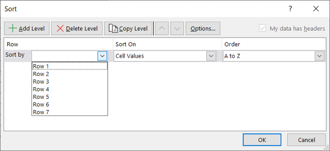
To filter data, select the range, click the "Filter" button, click on the drop-down arrows, and display only the data that meets your chosen criteria.

3 Autofit the Data in Cells

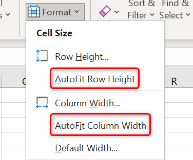
When entering long text or numbers into cells that don’t fit within their default size, the data either gets cut off or spills into neighboring cells. Excel’s autofit feature solves this issue by automatically adjusting the cell’s width and height to fit the content. This eliminates the need to resize it manually. This also makes your spreadsheets more visually appealing.

Since it's a frequently used feature, you must learn how to use it. To quickly autofit content, double-click the boundary between two column or row headers where data overlaps. Alternatively, go to the "Home" tab, click "Format," and choose "AutoFit Row Height" or "AutoFit Column Width."

4 Freeze Panes

Column and row headers provide context for the data, but they can quickly disappear from view when you scroll down or across a large spreadsheet. When I started using Excel, this was a constant frustration as I had to keep scrolling back to check the headers. Then, I found that Excel allows you to freeze specific rows and columns, keeping the headers always visible.

To freeze headers, go to the "View" tab, click "Freeze Panes," and select "Freeze Panes," "Freeze Top Row" or "Freeze First Column."

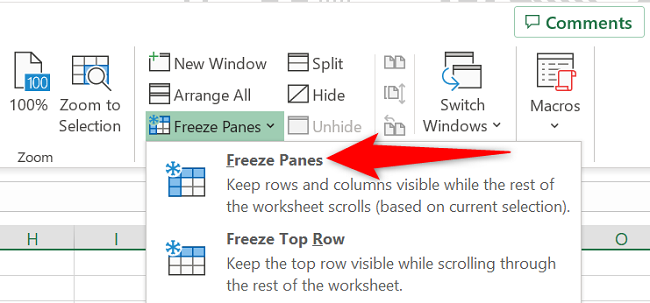
To freeze multiple rows or columns, select the cell just below the rows and to the right of the columns you want to lock, then go to "Freeze Panes" and choose "Freeze Panes" again. This will freeze everything above and to the left of your selected cell.

5 Lock Selected Cells From Being Edited

When sharing spreadsheets, especially with users having editing access, you must lock cells containing data you don’t want others to alter accidentally or intentionally. To lock specific cells in Excel, select all cells in the sheet, then hold the Ctrl key and highlight the ones you want to protect. This will deselect them from the current selection.

Next, press Ctrl+1, go to the "Protection" tab, and uncheck the "Locked" box. Finally, click "OK."

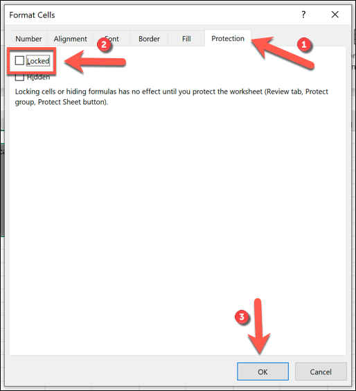
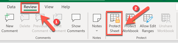
After that, go to the "Review" tab, open the "Protect" drop-down menu, select "Protect Sheet," and click "OK."

6 Learn Keyboard Shortcuts

Keyboard shortcuts eliminate the need to navigate tabs, search for options, or perform repetitive tasks. They allow you to move around your workbook without using a mouse or trackpad. So, familiarizing yourself with some of the useful keyboard shortcuts can really save you time and manual effort.

For example, Ctrl+Page Up/Down lets you switch between sheets, Ctrl+G opens the "Go To" dialog for quick navigation, and Ctrl+H launches the "Find and Replace" tool to update data. Similarly, Ctrl+` (backtick) displays formulas instead of results for easy verification; Ctrl+Space selects an entire column, and Shift+Space selects an entire row.

Pressing F4 repeats your last action, and you can manage cell formatting by pressing Ctrl+1. You should also explore other useful shortcuts to streamline your workflow in Excel.

7 Understand Cell References

You must use the correct cell references—relative, absolute, and mixed—to accurately point to specific cells and ranges as they directly affect the precision of your calculations.

Relative references (e.g., A1) adjust automatically when you copy or move a formula to a new location. For example, if you create a formula in B1 that refers to A1 and then copy it to B2, it will change to reference A2. In contrast, absolute references (e.g., $A$1) remain constant regardless of where the formula is copied or moved.

Mixed references let you lock the row or the column while keeping the other part flexible. For example, A$1 will lock row 1 while allowing the column to adjust when the formula is copied.

8 Error Checking and Troubleshooting Tools

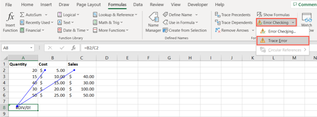
When encountering errors in formulas or inputs, you must know how to identify, understand, and resolve them. Excel provides various tools to help with troubleshooting. For example, if a cell displays an error like #DIV/0!, #NAME?, or #VALUE!, you can click the green triangle in the top-left corner of the cell to get an explanation and suggestions for fixing the error.

If the issue relates to cell references, tools like Trace Precedents and Trace Dependents can help you track down the problem. Also, the "Evaluate Formula" tool allows you to step through formulas one step at a time to identify issues more quickly. Functions like ISERROR and IFERROR are also helpful in troubleshooting errors within your spreadsheet.

Likewise, Excel’s built-in error-checking tool, available under Formulas > Error Checking > Trace Error, can scan your worksheet for common formula errors and help you fix them.

These are some of the frequently used Excel features you should know as a beginner. However, learning Excel is an ongoing process; it takes years to master many of its features, and there will always be more to discover. Make it a habit to regularly explore Excel features and learn something new every day.