How to Use the TREND Function in Excel

One way to give more meaning to your numbers in Excel is to understand the trends lying behind them, and being able to do so is crucial in today's ever-changing world. Using Excel's TREND function will help you identify patterns in previous and current data, as well as project future movements.

What Is TREND Used For?

The TREND function has three primary uses in Excel:

Calculate a linear trend through a set of existing data, Predict future figures based on existing data, and Create a trendline in a chart that helps you forecast future data.

TREND can be used to measure performance or forecast finances in the workplace, and you can also use it on your personal spreadsheets to track your spending, predict how many goals your team will score, and a host of other uses.

How Does TREND Work?

Excel's TREND function calculates what would be the line of best fit on a chart using the least-squares method.

The line of best fit is calculated using the equation

y = mx + b

where

y is the dependent variable, m is the gradient (steepness) of the trendline, x is the independent variable, and b is the y-intercept (where the trendline crosses the y-axis)

While it's not essential to know this information, it's handy for choosing what you want to include in your TREND formula syntax.

What Is the Syntax for TREND?

Now that you understand what a trendline is and how it's calculated, let's look at the Excel formula.

TREND(known_y's,known_x's,new_x's,const)

where

known_y's (required) are the dependent variables you already have that will help Excel calculate the trend. Without these, Excel can't calculate a trend, so your input would result in an error message. These values would sit on the y-axis on a column chart. known_x's (optional) are the independent variables that would sit on the x-axis on a column chart, and these must be the same length (number of cells) as the known_y's reference. new_x's (optional) is one or more sets of new independent variables on the x-axis for which you want Excel to calculate the trend. This tells Excel how many new y-values you want to add to your data. const (optional) is a logical value that defines the intercept (value b in y = mx + b). FALSE forces the trendline to pass through 0 on the x-axis, while TRUE means the intercept is applied normally. Omitting this value is the same as inserting TRUE (normal).

Calculating Your Existing Data's Trend

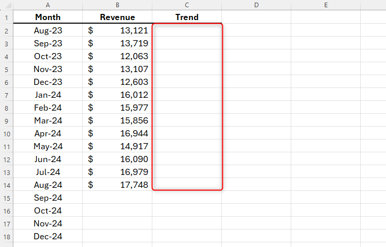
It's now time to put this into action. In the example below, we have the revenue for each of the past few months, and we want to work out the trend for this data.

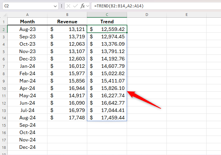
To do this, we need to type the following formula into cell C2:

=TREND(B2:B14,A2:A14)

where B2:B14 are the known y-values, and A2:A14 are the known x-values. We don't need any new x-values at this point, as we aren't creating any forecast revenue data. Also, we don't need a const value, as setting the y-intercept at 0 would yield inaccurate data.

Press Enter after typing your formula, and see that the trend is displayed as an array.

Predicting Future Figures

Now that we have an idea of the trend of our data, we're ready to use this information to forecast the following months. In other words, we want to complete the trend column in our table.

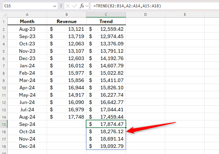
So, in cell C15, we will type

=TREND(B2:B14,A2:A14,A15:A18)

where B2:B14 are the known y-values, A2:A14 are the known x-values, and A15:A18 are the new x-values for the predictive trend we're calculating. We haven't specified a const value, as we want the y-intercept to calculate normally.

Press Enter to see the outcome.

Using TREND With Charts

Now that we have all the data up to the current date, as well as the predictive trendline for the coming month, we're ready to see how this looks on a chart.

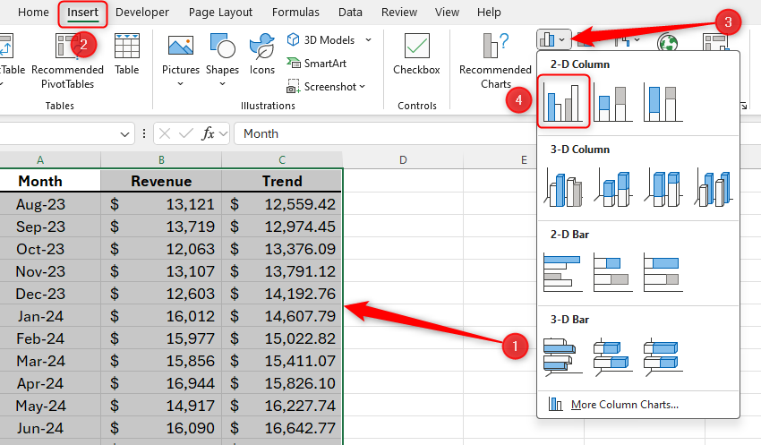
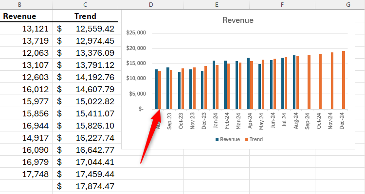
Select all the data in your table, including the headings, and click "2D Clustered Column Chart" in the Insert tab on the ribbon.

At first, you will see both the independent variable (in our case, revenue) and the trendline on the x-axis, but we want the trend data to show as a line.

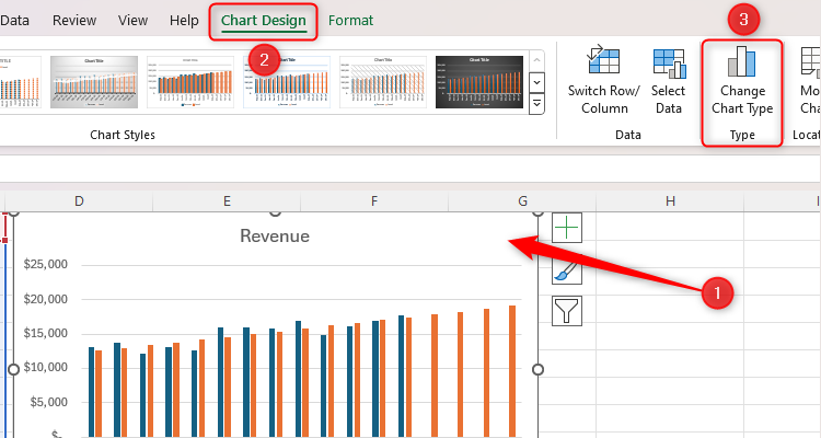
To amend this, click anywhere on the chart, and select "Change Chart Type" in the Chart Design tab on the ribbon.

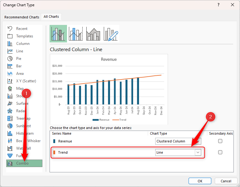
Then, select the "Combo" chart type, and make sure your trendline is set to "Line."

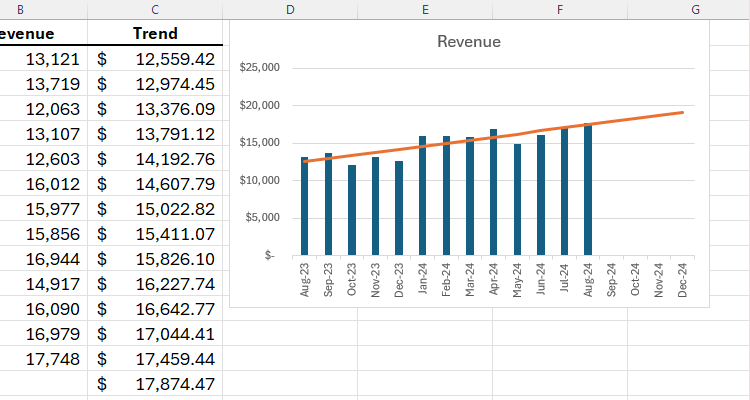
Then, click "OK" to see your new chart with the trendline showing as you would expect, including as a projection for future months. We've also clicked "+" in the corner of our chart to remove the data legend, as it's not necessary for this chart.

If you aren't looking to see future projections in your data, you can add a trendline to your chart without using the TREND function. Simply hover your cursor over the chart, click the "+" in the top-right corner, and check "Trendline." Another way to see trends is to use Excel's Sparklines, which you can find in the Insert tab on the ribbon.